注意力机制系列可以参考前面的一文:
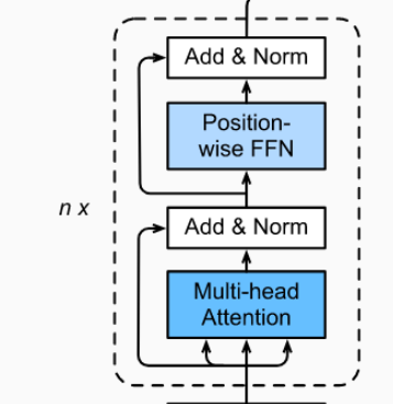
Transformer Block
BERT中的点积注意力模型
公式:
$$ \text{Attention}(\boldsymbol{Q},\boldsymbol{K},\boldsymbol{V}) = \text{softmax}(\frac{\boldsymbol{Q}\boldsymbol{K}^T}{\sqrt{d_k}})\boldsymbol{V} $$代码:
class Attention(nn.Module): |
在 𝑠𝑒𝑙𝑓 𝑎𝑡𝑡𝑒𝑛𝑡𝑖𝑜𝑛 的计算过程中, 通常使用 𝑚𝑖𝑛𝑖 𝑏𝑎𝑡𝑐ℎ 来计算, 也就是一次计算多个句子,多句话得长度并不一致,因此,我们需要按照最大得长度对短句子进行补全,也就是padding零,但这样做得话,softmax计算就会被影响,$e^0=1$也就是有值,这样就会影响结果,这并不是我们希望看到得,因此在计算得时候我们需要把他们mask起来,填充一个负无穷(-1e9这样得数值),这样计算就可以为0了,等于把计算遮挡住。
多头自注意力模型
公式:
$$ \text{MultiHead}(Q,K,V) = \text{Concat}(\text{head1},...,\text{head}_h)\boldsymbol{W}^O $$ $$ \text{head}_i = \text{Attention}(\boldsymbol{Q}\boldsymbol{W}_i^Q,\boldsymbol{K}\boldsymbol{W}_i^K,\boldsymbol{V}\boldsymbol{W}_i^V) $$ $$ \text{Attention}(\boldsymbol{Q},\boldsymbol{K},\boldsymbol{V}) = \text{softmax}(\frac{\boldsymbol{Q}\boldsymbol{K}^T}{\sqrt{d_k}})\boldsymbol{V} $$Attention Mask
代码:
class MultiHeadedAttention(nn.Module): |
Position-wise FFN
Position-wise FFN 是一个双层得神经网络,在论文中采用ReLU做激活层:
公式:
$$
\text{FFN}(x) = \text{max}(0, x\boldsymbol{W}_1 + b_1)\boldsymbol{W}_2 + b_2
$$
注:在 google github中的BERT的代码实现中用Gaussian Error Linear Unit代替了RelU作为激活函数
代码:class PositionwiseFeedForward(nn.Module):
def __init__(self, d_model, d_ff, dropout=0.1):
super(PositionwiseFeedForward, self).__init__()
self.w_1 = nn.Linear(d_model, d_ff)
self.w_2 = nn.Linear(d_ff, d_model)
self.dropout = nn.Dropout(dropout)
self.activation = GELU()
def forward(self, x):
return self.w_2(self.dropout(self.activation(self.w_1(x))))
class GELU(nn.Module):
"""
Gaussian Error Linear Unit.
This is a smoother version of the RELU.
Original paper: https://arxiv.org/abs/1606.08415
"""
def forward(self, x):
return 0.5 * x * (1 + torch.tanh(math.sqrt(2 / math.pi) * (x + 0.044715 * torch.pow(x, 3))))
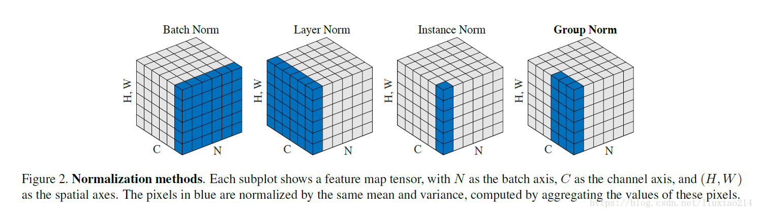
Layer Normalization
LayerNorm实际就是对隐含层做层归一化,即对某一层的所有神经元的输入进行归一化(沿着通道channel方向),使得其加快训练速度:
层归一化公式:
$$
\sigma^l = \sqrt{\frac{1}{\boldsymbol{H}}\sum_{i=1}^{\boldsymbol{H}}(x_i^l-\mu^l)^2} \\
\mu^l = \frac{1}{\boldsymbol{H}}\sum_{i=1}^{\boldsymbol{H}}x_i^l \\
x^l = w_i^l h^l
$$
$l$表示第L层,H 是指每层的隐藏单元数(hidden unit),$\mu$表示平均值,$\sigma$表示方差, $\alpha$表示表征向量,$w$表示矩阵权重。
$$
\text{LayerNorm}(x) = \alpha \odot \frac{x - \mu}{\sqrt{\sigma^2+\epsilon}} + \beta
$$
注:$\odot$表示元素相乘
其中,$\alpha$和$\beta$、$\epsilon$为超参数。
代码:class LayerNorm(nn.Module):
"Construct a layernorm module (See citation for details)."
def __init__(self, features, eps=1e-6):
super(LayerNorm, self).__init__()
self.a_2 = nn.Parameter(torch.ones(features))
self.b_2 = nn.Parameter(torch.zeros(features))
self.eps = eps
def forward(self, x):
# mean(-1) 表示 mean(len(x)), 这里的-1就是最后一个维度,也就是最里面一层的维度
mean = x.mean(-1, keepdim=True)
std = x.std(-1, keepdim=True)
return self.a_2 * (x - mean) / (std + self.eps) + self.b_2
残差连接
残差连接就是图中Add+Norm层。每经过一个模块的运算, 都要把运算之前的值和运算之后的值相加, 从而得到残差连接,残差可以使梯度直接走捷径反传到最初始层。
残差连接公式:
$$
\boldsymbol{y} = f(\boldsymbol{x}) + \boldsymbol{x}
$$
X 表示输入的变量,实际就是跨层相加。
代码:class SublayerConnection(nn.Module):
"""
A residual connection followed by a layer norm.
Note for code simplicity the norm is first as opposed to last.
"""
def __init__(self, size, dropout):
super(SublayerConnection, self).__init__()
self.norm = LayerNorm(size)
self.dropout = nn.Dropout(dropout)
def forward(self, x, sublayer):
"Apply residual connection to any sublayer with the same size."
# Add and Norm
return x + self.dropout(sublayer(self.norm(x)))
Transform Block
代码:class TransformerBlock(nn.Module):
"""
Bidirectional Encoder = Transformer (self-attention)
Transformer = MultiHead_Attention + Feed_Forward with sublayer connection
"""
def __init__(self, hidden, attn_heads, feed_forward_hidden, dropout):
"""
:param hidden: hidden size of transformer
:param attn_heads: head sizes of multi-head attention
:param feed_forward_hidden: feed_forward_hidden, usually 4*hidden_size
:param dropout: dropout rate
"""
super().__init__()
# 多头注意力模型
self.attention = MultiHeadedAttention(h=attn_heads, d_model=hidden)
# PFFN
self.feed_forward = PositionwiseFeedForward(d_model=hidden, d_ff=feed_forward_hidden, dropout=dropout)
# 输入层
self.input_sublayer = SublayerConnection(size=hidden, dropout=dropout)
# 输出层
self.output_sublayer = SublayerConnection(size=hidden, dropout=dropout)
self.dropout = nn.Dropout(p=dropout)
def forward(self, x, mask):
x = self.input_sublayer(x, lambda _x: self.attention.forward(_x, _x, _x, mask=mask))
x = self.output_sublayer(x, self.feed_forward)
return self.dropout(x)
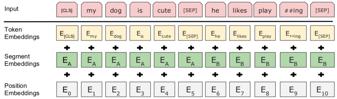
Embedding嵌入层
Embedding采用三种相加的形式表示:
代码:class BERTEmbedding(nn.Module):
"""
BERT Embedding which is consisted with under features
1. TokenEmbedding : normal embedding matrix
2. PositionalEmbedding : adding positional information using sin, cos
3. SegmentEmbedding : adding sentence segment info, (sent_A:1, sent_B:2)
sum of all these features are output of BERTEmbedding
"""
def __init__(self, vocab_size, embed_size, dropout=0.1):
"""
:param vocab_size: total vocab size
:param embed_size: embedding size of token embedding
:param dropout: dropout rate
"""
super().__init__()
self.token = TokenEmbedding(vocab_size=vocab_size, embed_size=embed_size)
self.position = PositionalEmbedding(d_model=self.token.embedding_dim)
self.segment = SegmentEmbedding(embed_size=self.token.embedding_dim)
self.dropout = nn.Dropout(p=dropout)
self.embed_size = embed_size
def forward(self, sequence, segment_label):
x = self.token(sequence) + self.position(sequence) + self.segment(segment_label)
return self.dropout(x)
位置编码(Positional Embedding)
位置嵌入的维度为 [𝑚𝑎𝑥 𝑠𝑒𝑞𝑢𝑒𝑛𝑐𝑒 𝑙𝑒𝑛𝑔𝑡ℎ, 𝑒𝑚𝑏𝑒𝑑𝑑𝑖𝑛𝑔 𝑑𝑖𝑚𝑒𝑛𝑠𝑖𝑜𝑛] , 嵌入的维度同词向量的维度, 𝑚𝑎𝑥 𝑠𝑒𝑞𝑢𝑒𝑛𝑐𝑒 𝑙𝑒𝑛𝑔𝑡ℎ 属于超参数, 指的是限定的最大单个句长.
公式:
$$ \boldsymbol{P}_{i,2j} = \text{sin}(\frac{i}{10000^{2j/d}}) $$ $$ \boldsymbol{P}_{i,2j+1} = \text{sin}(\frac{i}{10000^{2j/d}}) $$ $$ \boldsymbol{H} = \boldsymbol{X} + \boldsymbol{P}, \\ \boldsymbol{X} \in \Bbb{R}, \boldsymbol{P} \in \Bbb{R} $$其所绘制的图形:
代码:class PositionalEmbedding(nn.Module):
def __init__(self, d_model, max_len=512):
super().__init__()
# Compute the positional encodings once in log space.
pe = torch.zeros(max_len, d_model).float()
pe.require_grad = False
position = torch.arange(0, max_len).float().unsqueeze(1)
div_term = (torch.arange(0, d_model, 2).float() * -(math.log(10000.0) / d_model)).exp()
pe[:, 0::2] = torch.sin(position * div_term)
pe[:, 1::2] = torch.cos(position * div_term)
# 对数据维度进行扩充,扩展第0维
pe = pe.unsqueeze(0)
# 添加一个持久缓冲区pe,缓冲区可以使用给定的名称作为属性访问
self.register_buffer('pe', pe)
def forward(self, x):
return self.pe[:, :x.size(1)]
Segment Embedding
主要用来做额外句子或段落划分新够词,
这里加入了三个维度,分别是句子
开头【CLS】,下一句【STEP】,遮盖词【MASK】
例如: [CLS] the man went to the store [SEP] he bought a gallon of milk [SEP]
代码:class SegmentEmbedding(nn.Embedding):
def __init__(self, embed_size=512):
# 3个新词
super().__init__(3, embed_size, padding_idx=0)
Token Embedding
代码:class TokenEmbedding(nn.Embedding):
def __init__(self, vocab_size, embed_size=512):
super().__init__(vocab_size, embed_size, padding_idx=0)
BERT
class BERT(nn.Module): |
语言模型训练的几点技巧
BERT如何做到自训练的,一下是几个小tip,让其做到自监督训练:
Mask
随机遮盖或替换一句话里面任意字或词, 然后让模型通过上下文的理解预测那一个被遮盖或替换的部分, 之后做𝐿𝑜𝑠𝑠的时候只计算被遮盖部分的𝐿𝑜𝑠𝑠。
随机把一句话中 15% 的 𝑡𝑜𝑘𝑒𝑛 替换成以下内容:
- 1) 这些 𝑡𝑜𝑘𝑒𝑛 有 80% 的几率被替换成 【𝑚𝑎𝑠𝑘】 ;
- 2) 有 10% 的几率被替换成任意一个其他的 𝑡𝑜𝑘𝑒𝑛 ;
- 3) 有 10% 的几率原封不动.
让模型预测和还原被遮盖掉或替换掉的部分,损失函数只计算随机遮盖或替换部分的Loss。
代码:class MaskedLanguageModel(nn.Module):
"""
predicting origin token from masked input sequence
n-class classification problem, n-class = vocab_size
"""
def __init__(self, hidden, vocab_size):
"""
:param hidden: output size of BERT model
:param vocab_size: total vocab size
"""
super().__init__()
self.linear = nn.Linear(hidden, vocab_size)
self.softmax = nn.LogSoftmax(dim=-1)
def forward(self, x):
return self.softmax(self.linear(x))
预测下一句
代码:class NextSentencePrediction(nn.Module):
"""
2-class classification model : is_next, is_not_next
"""
def __init__(self, hidden):
"""
:param hidden: BERT model output size
"""
super().__init__()
self.linear = nn.Linear(hidden, 2)
# 这里采用了logsoftmax代替了softmax,
# 当softmax值远离真实值的时候梯度也很小,logsoftmax的梯度会更好些
self.softmax = nn.LogSoftmax(dim=-1)
def forward(self, x):
return self.softmax(self.linear(x[:, 0]))
损失函数
负对数最大似然损失(negative log likelihood),也叫交叉熵(Cross-Entropy)公式:
$$
E(t,y) = -\sum_i t_i \text{log}y_i
$$
代码:# 在Pytorch中 CrossEntropyLoss()等于NLLLoss+ softmax,因此如果用CrossEntropyLoss最后一层就不用softmax了
criterion = nn.NLLLoss(ignore_index=0)
# 2-1. NLL(negative log likelihood) loss of is_next classification result
next_loss = criterion(next_sent_output, data["is_next"])
# 2-2. NLLLoss of predicting masked token word
mask_loss = criterion(mask_lm_output.transpose(1, 2), data["bert_label"])
# 2-3. Adding next_loss and mask_loss : 3.4 Pre-training Procedure
loss = next_loss + mask_loss
语言模型训练
代码:class BERTLM(nn.Module):
"""
BERT Language Model
Next Sentence Prediction Model + Masked Language Model
"""
def __init__(self, bert: BERT, vocab_size):
"""
:param bert: BERT model which should be trained
:param vocab_size: total vocab size for masked_lm
"""
super().__init__()
self.bert = bert
self.next_sentence = NextSentencePrediction(self.bert.hidden)
self.mask_lm = MaskedLanguageModel(self.bert.hidden, vocab_size)
def forward(self, x, segment_label):
x = self.bert(x, segment_label)
return self.next_sentence(x), self.mask_lm(x)
云端部署BERT SERVICE
下载BERT预训练模型:
BERT-as-service架构:
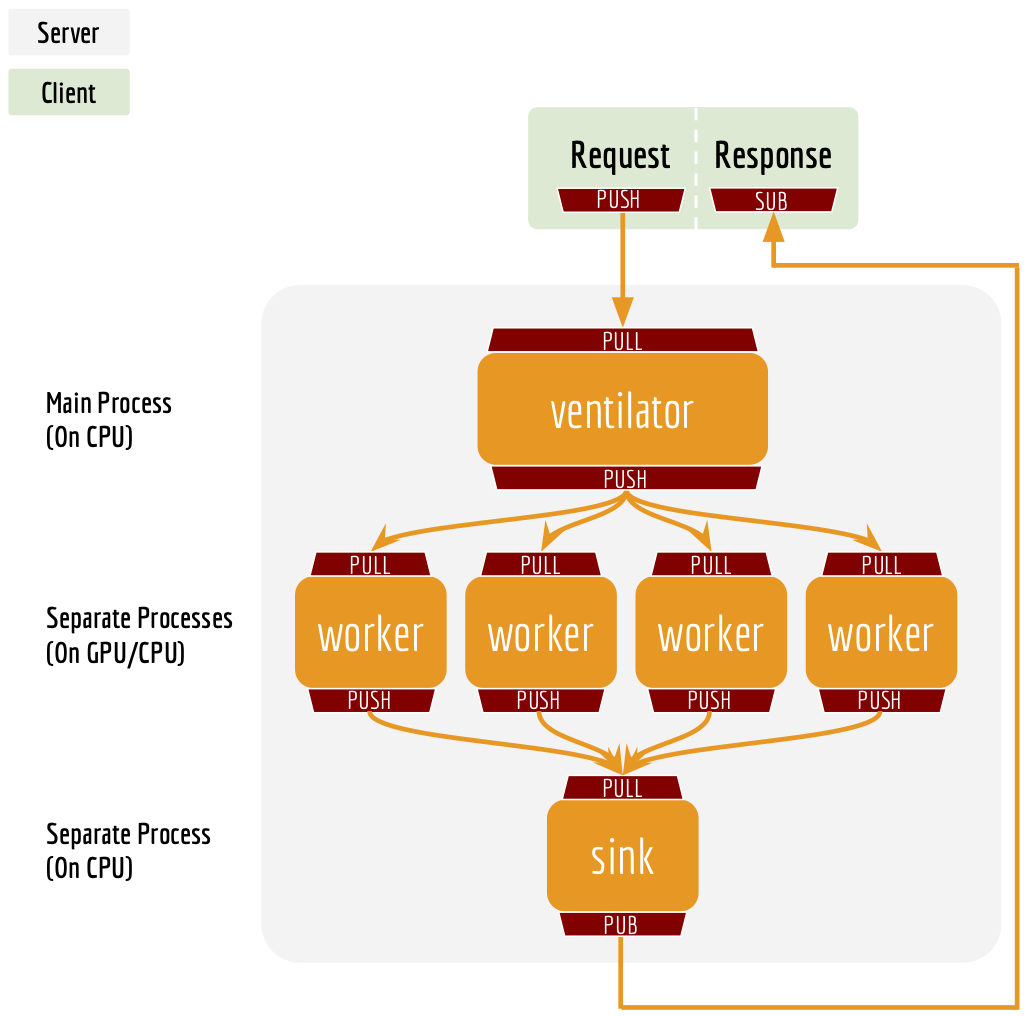
先建立service容器
搭建kubernetes服务
###